Introduction to graph algorithms: definitions and examples

This text introduces basic graph terminology, standard graph data structures, and three fundamental algorithms for traversing a graph in a systematic way.

You may also want to take a look at the Github yourbasic/graph repository. It’s a Go library with generic implementations of basic graph algorithms.

Definitions

A graph G consists of two types of elements: vertices and edges. Each edge has two endpoints, which belong to the vertex set. We say that the edge connects (or joins) these two vertices.

The vertex set of G is denoted V(G), or just V if there is no ambiguity.

An edge between vertices u and v is written as {u, v}. The edge set of G is denoted E(G), or just E if there is no ambiguity.

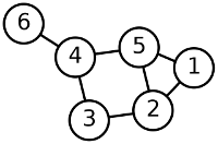
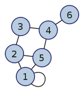
The graph in this picture has the vertex set V = {1, 2, 3, 4, 5, 6}. The edge set E = {{1, 2}, {1, 5}, {2, 3}, {2, 5}, {3, 4}, {4, 5}, {4, 6}}.

A self-loop is an edge whose endpoints is a single vertex. Multiple edges are two or more edges that join the same two vertices.

A graph is called simple if it has no self-loops and no multiple edges, and a multigraph if it does have multiple edges.

The degree of a vertex v is the number of edges that connect to v.

A path in a graph G = (V, E) is a sequence of vertices v₁, v₂, …, v_k, with the property that there are edges between v_i and v_i+1. We say that the path goes from v₁ to v_k. The sequence 6, 4, 5, 1, 2 is a path from 6 to 2 in the graph above. A path is simple if its vertices are all different.

A cycle is a path v₁, v₂, …, v_k for which k > 2, the first k - 1 vertices are all different, and v₁ = v_k. The sequence 4, 5, 2, 3, 4 is a cycle in the graph above.

A graph is connected if for every pair of vertices u and v, there is a path from u to v.

If there is a path connecting u and v, the distance between these vertices is defined as the minimal number of edges on a path from u to v.

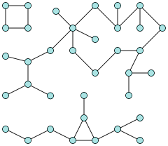
A connected component is a subgraph of maximum size, in which every pair of vertices are connected by a path. Here is a graph with three connected components.

Trees

A tree is a connected simple acyclic graph. A vertex with degree 1 in a tree is called a leaf.

Directed graphs

A directed graph or digraph G = (V, E) consists of a vertex set V and an edge set of ordered pairs E of elements in the vertex set.

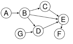
Here is a simple acyclic digraph (often called a DAG, “directed acyclic graph”) with seven vertices and eight edges.

Data structures

Adjacency matrix

An adjacency matrix is a |V|x|V|-matrix of integers, representing a graph G = (V, E).

• The vertices are number from 1 to |V|.
• The number at position (i, j) indicates the number of edges from i to j.

Here is an undirected graph and its symmetric adjacency matrix.

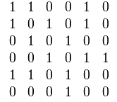
The adjacency matrix representation is best suited for dense graphs, graphs in which the number of edges is close to the maximal.

In a sparse graph, an adjacency matrix will have a large memory overhead, and finding all neighbors of a vertex will be costly.

Adjacency list

The adjacency list graph data structure is well suited for sparse graphs. It consists of an array of size |V|, where position k in the array contains a list of all neighbors to k.

Note that the “neighbor list” doesn’t have to be an actual list. It could be any data structure representing a set of vertices. Hash tables, arrays or linked lists are common choices.

Search algorithms

Depth-first search

Depth-first search (DFS) is an algorithm that visits all edges in a graph G that belong to the same connected component as a vertex v.

Algorithm DFS(G, v)
    if v is already visited
        return        
    Mark v as visited.
    // Perform some operation on v.
    for all neighbors x of v
        DFS(G, x)

Before running the algorithm, all |V| vertices must be marked as not visited.

Time complexity

To compute the time complexity, we can use the number of calls to DFS as an elementary operation: the if statement and the mark operation both run in constant time, and the for loop makes a single call to DFS for each iteration.

Let E' be the set of all edges in the connected component visited by the algorithm. The algorithm makes two calls to DFS for each edge {u, v} in E': one time when the algorithm visits the neighbors of u, and one time when it visits the neighbors of v.

Hence, the time complexity of the algorithm is Θ(|V| + |E'|).

Breadth-first search

Breadth-first search (BFS) also visits all vertices that belong to the same component as v. However, the vertices are visited in distance order: the algorithm first visits v, then all neighbors of v, then their neighbors, and so on.

Algorithm BFS(G, v)
    Q ← new empty FIFO queue
    Mark v as visited.
    Q.enqueue(v)
    while Q is not empty
        a ← Q.dequeue()
        // Perform some operation on a.
        for all unvisited neighbors x of a
            Mark x as visited.
            Q.enqueue(x)

Before running the algorithm, all |V| vertices must be marked as not visited.

Time complexity

The time complexity of BFS can be computed as the total number of iterations performed by the for loop.

Let E' be the set of all edges in the connected component visited by the algorithm. For each edge {u, v} in E' the algorithm makes two for loop iteration steps: one time when the algorithm visits the neighbors of u, and one time when it visits the neighbors of v.

Hence, the time complexity is Θ(|V| + |E'|).

Dijkstra’s algorithm

Dijkstra’s algorithm computes the shortest path from a vertex s, the source, to all other vertices. The graph must have non-negative edge costs.

The algorithm returns two arrays:

• dist[k] holds the length of a shortest path from s to k,
• prev[k] holds the previous vertex in a shortest path from s to k.

Algorithm Dijkstra(G, s)
    for each vertex v in G
        dist[v] ← ∞
        prev[v] ← undefined
    dist[s] ← 0

    Q ← the set of all nodes in G
    while Q is not empty
        u ← vertex in Q with smallest distance in dist[]
        Remove u from Q.
        if dist[u] = ∞
            break
        for each neighbor v of u
            alt ← dist[u] + dist_between(u, v)
            if alt < dist[v]
                dist[v] ← alt
                prev[v] ← u

    return dist[], prev[]

Time complexity

To compute the time complexity we can use the same type of argument as for BFS.

The main difference is that we need to account for the cost of adding, updating and finding the minimum distances in the queue. If we implement the queue with a heap, all of these operations can be performed in O(log |V|) time.

This gives the time complexity O((|E| + |V|)log|V|).

Share this page: